Understanding Big O Notation

Programmers, have you heard people say things like "this algorithm is Big O of N", and wondered what that meant?

It may sound intimidating, but the basic idea is both simple and useful. I don't have a CS background and learned this fairly recently, so let me give you a breakdown for beginners.

Orders of Growth

Every term like "Big O of (something)" describes an "order of growth". We're describing how an algorithm scales: as we throw larger inputs at it, how much more work does it have to do?

The size of the input could be "how many items are in a list that we want to sort?", or "how many web pages do we need to look through to find a search term?" Big O analysis answers questions like, "if we double the number of items, about how much more work do we have to do? Twice as much? A hundred times as much? Just one more step?"

Suppose we graph the scalability of some algorithms. On the X axis, we put the size of the inputs, and on the Y axis, the amount of work we have to do. They might look like this.

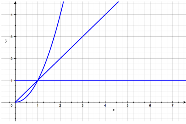
On a graph like this, you can distinguish orders of growth with one question: "How is the curve shaped?" We don't care about angle, and we don't care about position. When we're thinking about orders of growth, we gloss over a lot of details that we might care about otherwise.

Let's look at an example of each of these three kinds of curves.

Imagine we're running a conference, and we want to make sure that everyone feels welcome. How can we do that?

Handshakes

"I know", I say. "Handshakes. I'll walk around and personally greet everyone."

If we think of that as an algorithm and graph its performance, it looks like this:

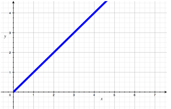
The amount of work that I have to do is always equal to the number of people, because 100 people need 100 handshakes. The code equivalent of this is a simple loop:

#!ruby
people.each do |person|
  greet(person)
end

Now suppose I want to be even friendlier. When I shake each person's hand, I want to take a few seconds to chat with them, get to know them, answer questions, etc. That's very nice, but if we graph it, we'll see that our line has a steeper slope, reflecting the fact that each attendee now requires more work than before. That's a change in angle.

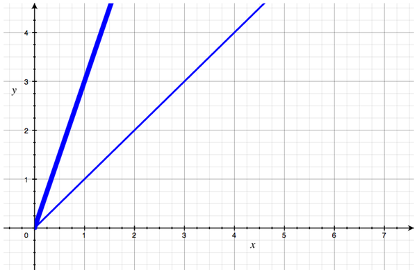
Alternately, suppose I stay with simple handshakes, but because I'm a bit of an introvert, I need a minute to psyche myself up before I start shaking hands. That graph looks something like this:

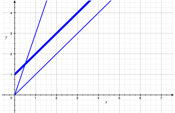
The slope is the same as the first one, but we've shifted the line upwards to show that for, say, 2 people, I have to do 3 units of work, since my preparation took 1 unit. The line's angle hasn't changed, but its position has.

Now, in absolute terms, each of these handshake algorithms performs differently. But in Big O terms, they're all the same: they are all linear, or O(N). Each of them has a shape that we can roughly describe as "a straight line with some slope". And that's all we care about. We don't care about angle, and we don't care about location; we only care about shape.

The reason is that, as I said, Big O is about scalability, and each of these scales in the same way: one more person means one more handshake; each new input adds the same amount of work as the last one did. That's why the line doesn't curve.

Introductions

Now imagine I do something different. Instead of just shaking hands, I decide to make introductions. I want every person at the conference to meet everyone else, so I introduce them. "Carla, this is Robert. Robert, Carla. Carla, this is Angie..."

The code equivalent of this is two nested loops:

#!ruby
people.each do |person|
  people.each do |other_person|
    introduce(person, other_person)
  end
end

That graph looks something like this:

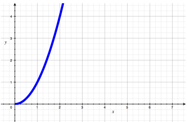
In this case, we do not have a straight line; the graph curves upward sharply, getting steeper and steeper. Why? Because this time, each additional attendee does not add a fixed amount of work. The eleventh person to show up only has to be introduced to ten people, but the one hundredth person needs ninety-nine introductions. Each input adds more work than the last.

This algorithm would be classified as O(N2), because for 10 people we need roughly 100 introductions, but for 100 people we need roughly 10,000 introductions. (I say "roughly" because, in reality, some of those introductions would be pointless, like introducing Alice to herself, or introducing Bob to Alice when we've already introduced Alice to Bob. But we do have 10,000 introductions to consider making.) In general, for N people, we need about N2 introductions.

Obviously, introductions will take a long time unless we have a very small group.

Wave

Now imagine we expect a lot of people, and we know we won't have time for introductions or handshakes. So we have a new idea: a wave. At the start of the conference, I just stand up on stage, wave at the crowd, and say some friendly words. "Hi, everyone! We're glad you're here!"

The code equivalent of that has no loop:

#!ruby
greet(people)

That algorithm is O(1), and the graph looks like this:

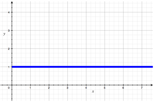
This shape looks a lot like our linear graph, but there's no angle; the line is flat.

Remember that N represents the number of inputs; in this case, how many people are at the conference. And notice that in the description O(1), the letter N does not appear. That's because it's irrelevant. It doesn't matter to me whether there are 10 people or 10 thousand; I can wave and say "hello" in the same amount of time. Each additional input adds no work at all. That's why O(1) is also called "constant time"; the amount of time it takes never changes.

This is beautiful. This is the holy grail of scalability. With an O(1) algorithm, you can increase your inputs forever and never bog down.

Scalability == Feasibility

Big O notation is about scalability, but at some point, it's also about feasibility. Maybe you can solve a problem when you have just a few inputs, but practically speaking, can you continue solving it for bigger inputs?

As a dramatic example, consider the Traveling Salesman problem. This is a famous problem in computer science, and it goes like this.

Suppose you have a list of cities that you need to visit on a business trip. You want to visit each one once and return to your home city. And you want to take the shortest route possible.

The brute force solution to this problem would be to first calculate every possible travel plan:

• New York, then London, then Bangalore...
• Bangalore, then Sydney, then Hong Kong...

...then sort them by distance traveled and pick the best one. But that solution is O(N!) ("O of N Factorial"). That means that for 3 cities, you have to consider (3 x 2 x 1) possible travel paths to solve it; for 4 cities, you have to consider (4 x 3 x 2 x 1) paths, and so forth.

This grows very quickly. It's hard for us to wrap our minds around this rate of growth. Let's see how you do at estimating it.

Suppose I tell you that with a certain computer, I can solve this problem for 5 cities in 0.12 seconds. How long will it take me to solve for 22 cities?

Go ahead. Make a guess.

...

Done? The answer is crazy: it would take about 35 billion years!

And that helps us see why this stuff matters. If you're dealing with an O(N!) algorithm, you want to know it.

For example, imagine that you work at a travel site, and someone suggests this as a feature. "Let's help people plan their trips!" OK, you might say. We can offer that feature... for 3 cities. We can offer that feature for 5 cities. But don't try to offer it for 10 cities, because the user will have taken their trip and come home before we find the optimum answer. And don't try to offer it for 22 cities, because the server farm will melt, civilization will collapse and the sun will burn out, and we still won't know the best route for their trip.

Theoretically, we can solve the problem, but practically, we can't; it just takes too long.

Hand-wavey for a reason

I said at the beginning that when we graph how an algorithm scales and want to know its order of growth, we only care about shape, not angle or location. We get really hand-wavey about those kinds of details, and others, too.

For example, suppose we write a script that sends out one email to each person on a list. Suppose it takes us 100 steps to create each person's email, and 200 steps to connect to a server and send them all. So if we have N people to send to, it will take us (100 * N) + 200 steps to finish the job.

In Big O terms, we'd just call that O(N), throwing away the 100 * (which is slope) and the + 200 (which is position; it shifts the curve upward on the graph). We discard them for a couple of reasons.

First, because they're not essential to the algorithm. We said that it takes 100 steps to build each email and 200 steps to send them all, but that could vary; maybe if we wrote the code differently, or used a different programming language, or used a different kind of computer chip, there would be more or fewer actual CPU instructions to execute. It's an "implementation detail"; not a characteristic of our algorithm, but of the particular way we happen to implement it. What won't change is the fact that we have to do some amount of work for each recipient.

Second, because we know that the category we're in matters more for scaling than the exact number of steps. In the long run - if N is positive and keeps getting larger - any O(1) algorithm will beat any O(N) algorithm, any O(N) algorithm will beat any O(N2) algorithm, and so on.

We can prove this. Suppose we have an algorithm that takes some flavor if N steps. Lets try to make that a big number; we'll say it takes 10,000 * N steps. Compare it to an algorithm that takes some flavor of N2 steps. Let's try to make that a small number: we'll say it takes N2 / 10,000 steps. To see that N2 will be worse in the long run, just set 10,000 * N = N2 / 10,000 and solve for N. I rigged this example to make the math dead simple.

# our starting equation...
10,000 * N          = N * N / 10,000

# multiply both sides by 10,000...
100,000,000 * N     = N * N

# divide both sides by N...
100,000,000         = N

So when N reaches 100 million, an algorithm that takes N2 / 10,000 and an algorithm that takes 10,000 * N steps will both take the same number of steps: 1 trillion (10¹²). After that, the one with N2 will take more, because it grows faster. For example, add 1 to N and we see that 10,000 * N = 1,000,000,010,000, but N2 / 10,000 = 1,000,000,020,000. As N grows, the gap will keep getting larger. If we graph these two curves, they cross at 100 million (10⁸) and never again.

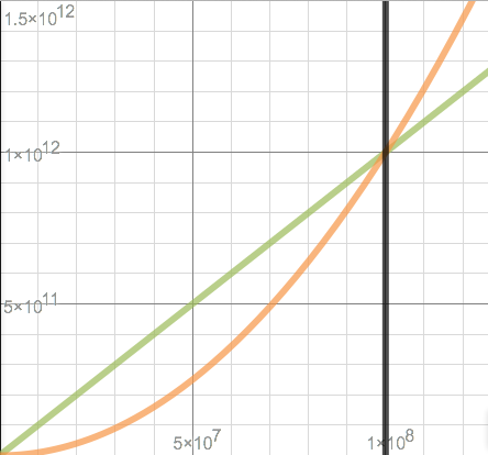
From there on out, the curve for N2 / 10,000 is always above the other one. It's worse in the long run, and we know exactly when the "long run" starts.

Yes, in this example, for values less than 100 million, N2 / 10,000 is better. So if you knew that you'd have small values of N, you should pick the algorithm that takes N2 / 10,000 steps. But Big O is a kind of "asymptotic analysis", asking about what happens as N moves toward infinity, so "the long run" is all it cares about.

Universally useful

I think you can see that Big O analysis is a practical tool. Another neat thing about it is that it's a universal tool, because algorithms are universal. For example, Quicksort is a way of sorting a list. You could do it in Ruby, Haskell, C, or by hand with a deck of cards. It will take an average of https://www.khanacademy.org/math/algebra2/logarithms-tutorial/logarithm_basics/v/logarithms">N * log2 N ("O of N log N") steps, no matter what language you're using or whether you're using a computer at all. Its "asymptotic order" (Big O category) is a characteristic of the universe, like 1 + 1 = 2.

That's why I'm excited about the topic, and why I want to learn more. For programmers, learning these nuggets of computer science is an investment that will keep paying off as long as we're solving problems.

Wrap-up

I haven't covered everything about Big O analysis, but I'm afraid I have told you everything I know. So let's recap quickly.

I said that the idea behind Big O notation is simple and useful. It's simple because it lets us ignore lots of details in favor of descriptions like "each conference attendee adds more work than the last" or "each one adds the same amount of work". And it's useful because it lets us answer questions like "can we actually solve this problem in a reasonable amount of time?"

Speaking of which, if you're a programmer, you probably use hashes (also known as dictionaries) all the time. Did you know that no matter how many items are in a hash, their lookup and insertion time never bogs down? It's O(1). How do they do that?

My next article diving into computer science topics will show you how to build your own hash data structure in Ruby and what makes hashes such a high-performing and versatile tool. Check back soon, or subscribe to the RSS feed, if you want to read more. (Update: here it is!)

Thanks to Aarti Parikh, Michael Gundlach, and Pat Shaughnessy for giving me feedback on a draft of this article. I'm very grateful for their insight. (Any remaining mistakes are my own, and I may revise this post from time to time.)